The dataset consists of three files (no file extension, but tab separated):
heatmap_genes A list of interesting genes to analyze (used in Figure 6b of the paper)
limma-voom_luminalpregnant-luminallactate: Differential expression results, including logFC, AveExpr, t-statistic, and p-value for all genes
limma-voom_normalised_counts: Normalized counts for genes across different samples
To simplify the analysis you can consider the following:
Read the files using read_tsv()
Clean column names with janitor::clean_names() to make them easier to work with
Combining relevant data frames using left_join() (limma-voom_luminalpregnant-luminallactate and limma-voom_normalised_counts share a common column)
Use select to remove columns you don’t need for analysis to get a better overview
Filter only significant genes (this tutorial defines them as p_value < 0.01 & abs(logFC) > 0.58)
It is a bit tricky to read in the data correctly, so if you need a hint, you can unfold the code below
Expand to see how to read the data
# Read all the files and clean the column namesheatmap_genes <-read_tsv("R/byod/solutions_for_my_datasets/data/heatmap_genes")DE_results <-read_tsv("R/byod/solutions_for_my_datasets/data/limma-voom_luminalpregnant-luminallactate")DE_results <- janitor::clean_names(DE_results)normalized_counts <-read_tsv("R/byod/solutions_for_my_datasets/data/limma-voom_normalised_counts")normalized_counts <- janitor::clean_names(normalized_counts)# combine tablesgenes <-left_join( DE_results, normalized_counts,by =c("entrezid", "symbol", "genename")) |>select(-entrezid, genename)
Questions
What are the top 20 most significantly differentially expressed genes?
Tip: Filter the genes based on p-value and log fold change, then order by p-value.
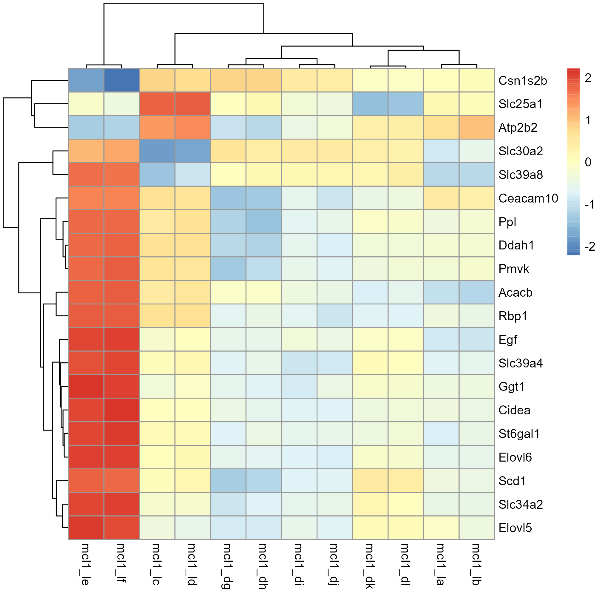
Create a heatmap of the top 20 most significant genes. How do the expression patterns differ between pregnant and lactating samples?
Checkout the pheatmap package for creating heatmaps.
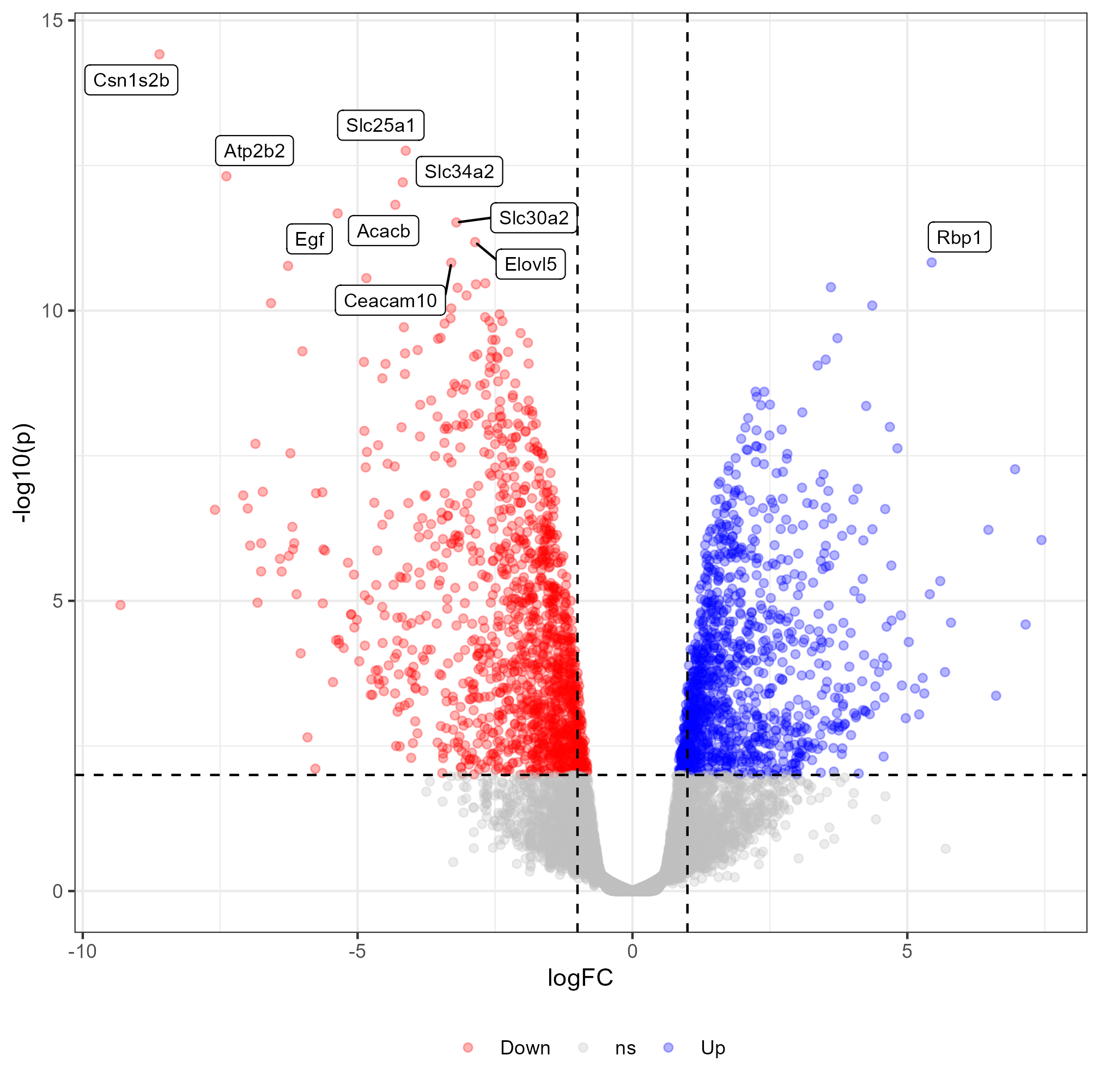
Create a volcano plot to visualize the differential expression results. How many genes are significantly up-regulated or down-regulated?
First create a simple volcano plot
Then you can try to label the 10 most significant genes in the volcano plot
Check my R script and/or this tutorial on how to create a volcano plot with ggplot
Perform a Principal Component Analysis (PCA) on the top 20 significant genes. What can you conclude about the separation of pregnant and lactating samples?
Tip: Use prcomp() for PCA and factoextra::fviz_pca_ind() for visualization.
Useful Functions
To complete these tasks, you may find the following R functions and packages helpful:
Data manipulation:
janitor::clean_names(): Clean column names
left_join(): Combine data frames
Statistical analysis:
scale(): Scale numeric variables
prcomp(): Perform Principal Component Analysis
Visualization:
pheatmap::pheatmap(): Create heatmaps (needs a matrix, so you need to reshape your data first into a matrix)
ggrepel::geom_text_repel(): Add non-overlapping labels to plots
factoextra::fviz_pca_ind(): Visualize PCA results
Other useful functions:
as.matrix(): Convert data frames to matrices
drop_na(): Drop rows with missing values (maybe needed for PCA because it doesn’t handle missing values)