Profiling R code

What are the speed & memory bottlenecks in my code?

• Use the profvis package

Profiling R code

You can profile a section of code like this:

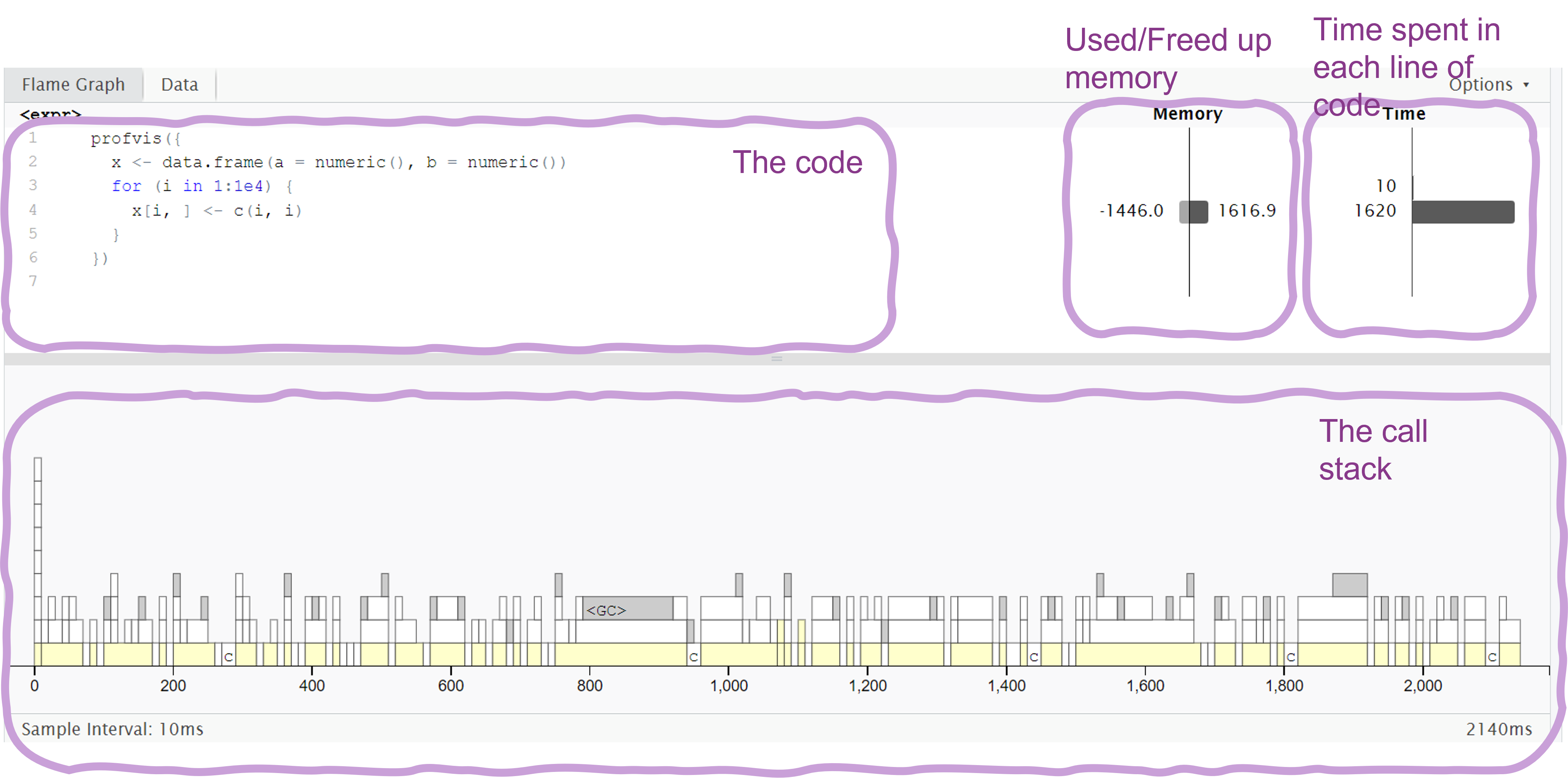
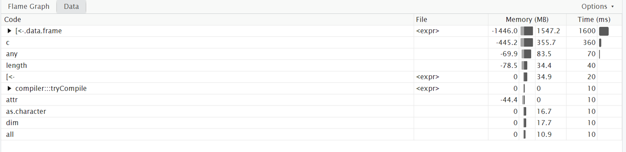
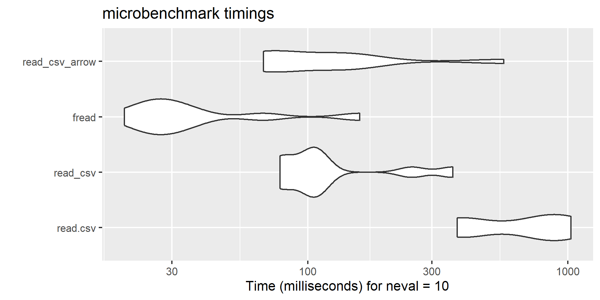
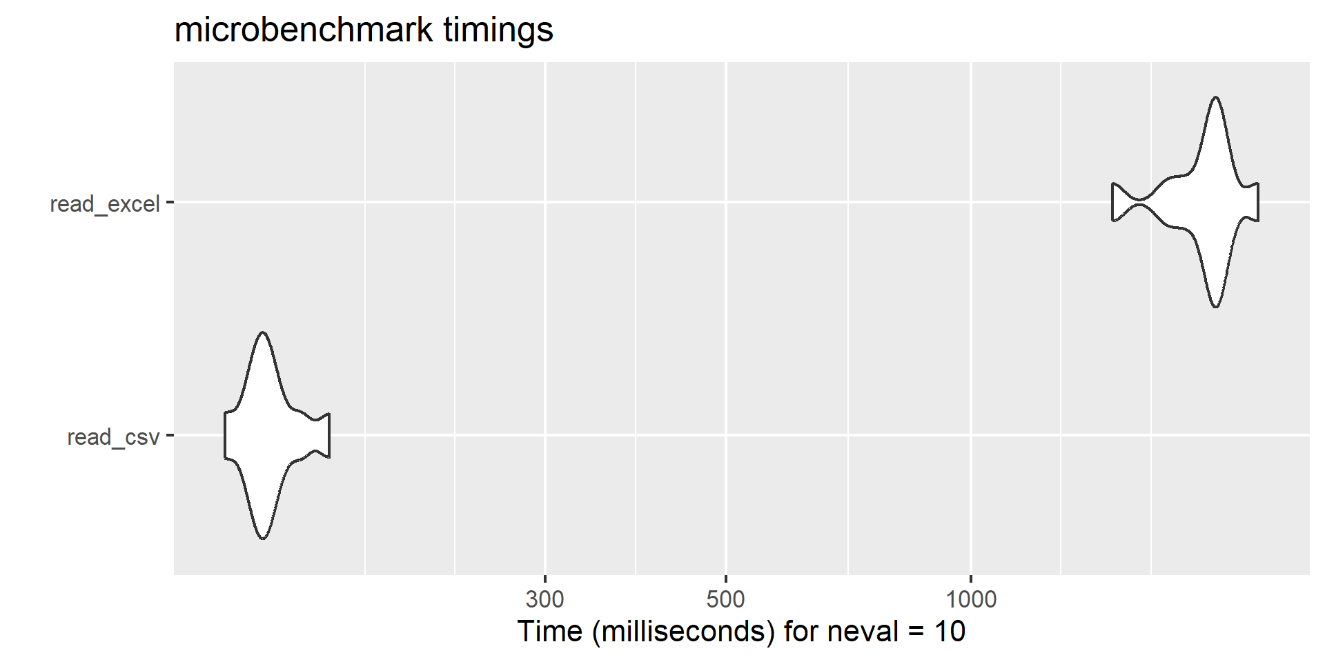
# install.packages("profvis")
library(profvis)

# Create a data frame with 150 columns and 400000 rows
df <- data.frame(matrix(rnorm(150 * 400000), nrow = 400000))

profvis({
  # Calculate mean of each column and put it in a vector
  means <- apply(df, 2, mean)

  # Subtract mean from each value in the table
  for (i in seq_along(means)) {
    df[, i] <- df[, i] - means[i]
  }
})

Profiling R code

Profvis flame graph shows time and memory spent in each line of code.

Profiling R code

Profvis data view for details on time spent in each function in the call stack.

Profiling R code

You can also interactively profile code in RStudio:

• Go to Profile -> Start profiling
• Now interactively run the code you want to profile
• Go to Profile -> Stop profiling to see the results

Benchmarking R code

Which version of the code is faster?

# Fill a data frame in a loop
f1 <- function() {
  x <- data.frame(a = numeric(), b = numeric())
  for (i in 1:1e4) {
    x[i, ] <- c(i, i)
  }
}

# Fill a data frame directly with vectors
f2 <- function() {
  x <- data.frame(a = 1:1e4, b = 1:1e4)
}

Benchmarking R code - the easy way

Use the tictoc package to get a quick overview of the time a section of code takes

# install.packages("tictoc")
library(tictoc)

tic()
f1()
toc()
#> 1.12 sec elapsed

tic()
f2()
toc()
#> 0 sec elapsed

Benchmarking R code

Use the microbenchmark package to compare the functions:

# install.packages("microbenchmark")
library(microbenchmark)

compare_functions <- microbenchmark(
  old = f1(),
  new = f2(),
  times = 10 # default is 100
)

compare_functions
#> Unit: microseconds
#>  expr     min        lq       mean     median      uq       max neval cld
#>   old 1063482 1107142.4 1139802.19 1135030.70 1176419 1210050.0    10  a 
#>   new      62      76.8     247.96     178.35     183    1267.8    10   b

library(ggplot2)
autoplot(compare_functions)

Benchmarking R code

Vectorize your code

• Vectors are central to R programming
• R is optimized for vectorized code
  • Implemented directly in C/Fortran
• Vector operations can often replace for-loops in R
• If there is a vectorized version of a function: Use it

Vectorize your code

Example: Calculate the log of every value in a vector and sum up the result

# A vector with 1 million values
x <- 1:1e6

microbenchmark(
  for_loop = {
    log_sum <- 0
    for (i in 1:length(x)) {
      log_sum <- log_sum + log(x[i])
    }
  },
  sum = sum(log(x)),
  times = 10
)
#> Unit: milliseconds
#>      expr     min      lq     mean  median      uq     max neval cld
#>  for_loop 58.7096 59.0902 59.96390 59.5209 60.4307 63.5593    10  a 
#>       sum 35.8210 36.6466 37.21634 37.0020 37.9745 38.8886    10   b

For-loops in R

• For-loops are relatively slow and it is easy to make them even slower with bad design

• Often they are used when vectorized code would be better

• For loops can often be replaced, e.g. by

  • Functions from the apply family (e.g. apply, lapply, …)
  • Vectorized functions (e.g. sum, colMeans, …)
  • Vectorized functions from the purrr package (e.g. map)

Cache variables

If you use a value multiple times, store it in a variable to avoid re-calculation

# A matrix with 1000 columns
x <- matrix(rnorm(10000), ncol = 1000)

microbenchmark(
  no_cache = apply(x, 2, function(i) mean(i) / sd(x)),
  cache = {
    sd_x <- sd(x)
    apply(x, 2, function(i) mean(i) / sd_x)
  }
)
#> Unit: milliseconds
#>      expr     min      lq      mean   median       uq      max neval cld
#>  no_cache 57.9128 60.9763 63.638999 62.88575 64.68335 111.1956   100  a 
#>     cache  3.3494  3.5692  3.676188  3.63415  3.71695   5.2457   100   b

Efficient workflow

• Prepare the data to be clean and concise for analysis
  • Helps to avoid unnecessary calculations
• Save intermediate results
  • Don’t re-run time-consuming steps if not necessary
• Use the right packages and functions

Read data

Example: Read csv data on worldwide emissions of greenhouse gases (~14000 rows, 7 cols).

• Base-R functions to read csv files are:
  • read.table
  • read.csv
• There are many alternatives to read data, e.g.:
  • read_csv from the readr package (tidyverse)
  • fread from the data.table package
  • read_csv_arrow from the arrow package

Read data

Compare some alternative reading functions

file_path_csv <- here::here("slides/data/ghg_ems_large.csv")

compare_input <- microbenchmark::microbenchmark(
  read.csv = read.csv(file_path_csv),
  read_csv = readr::read_csv(file_path_csv, progress = FALSE, show_col_types = FALSE),
  fread = data.table::fread(file_path_csv, showProgress = FALSE),
  read_csv_arrow = arrow::read_csv_arrow(file_path_csv),
  times = 10
)

autoplot(compare_input)

Use plain text data

Reading plain text is faster than excel files

file_path_xlsx <- here::here("slides/data/ghg_ems_large.xlsx")

compare_excel <- microbenchmark(
  read_csv = readr::read_csv(file_path_csv),
  read_excel = readxl::read_excel(file_path_xlsx),
  times = 10
)

autoplot(compare_excel)

Write data

• Base-R functions to write csv files are:
  • write.table
  • write.csv
• Faster alternatives are
  • write_csv from the readr package (tidyverse)
  • fwrite from the data.table package
  • write_csv_arrow from the arrow package

Efficient data manipulation

Different packages offer fast and efficient data manipulation and analysis:

• dplyr package has a C++ backend and is often faster than base R
• data.table package is fast and memory efficiency
  • Syntax is quite different from base R and tidyverse
• collapse package is a C++ based and specifically developed for fast data analysis
  • Works together with both tidyverse and data.table workflows
  • Many functions similar to base R or dplyr just with prefix “f” (e.g. fselect, fmean, …)
• arrow package for efficient reading, processing and writing of large datasets (even larger than RAM)

Summarize data by group

Example: Summarize mean carbon emissions from Electricity by Country

library(data.table)
library(dplyr)
library(collapse)

Summarize data by group

Example: Summarize mean carbon emissions from Electricity by Country

# 1. The data table way
# Convert the data to a data.table
setDT(ghg_ems)
summarize_dt <- function() {
  ghg_ems[, mean(Electricity, na.rm = TRUE), by = Country]
}

# 2. The dplyr way
summarize_dplyr <- function() {
  ghg_ems |>
    group_by(Country) |>
    summarize(mean_e = mean(Electricity, na.rm = TRUE))
}

# 3. The collapse way
summarize_collapse <- function() {
  ghg_ems |>
    fgroup_by(Country) |>
    fsummarise(mean_e = fmean(Electricity))
}

Efficient data manipulation

Example: Summarize mean carbon emissions from Electricity by Country

# compare the speed of all versions
microbenchmark(
  dplyr = summarize_dplyr(),
  data_table = summarize_dt(),
  collapse = summarize_collapse(),
  times = 10
)
#> Unit: microseconds
#>        expr    min     lq    mean  median     uq     max neval cld
#>       dplyr 2155.2 2179.4 3598.01 2262.65 2479.2 14360.4    10  a 
#>  data_table 1276.2 1329.9 2012.95 1474.85 1786.0  5818.1    10  ab
#>    collapse  157.1  177.2  382.28  203.65  235.0  1159.0    10   b

Select columns

Example: Select columns Country, Year, Electricity, Transportation

microbenchmark(
  dplyr = select(ghg_ems, Country, Year, Electricity, Transportation),
  data_table = ghg_ems[, .(Country, Electricity, Transportation)],
  collapse = fselect(ghg_ems, Country, Electricity, Transportation),
  times = 10
)
#> Unit: microseconds
#>        expr   min    lq   mean median    uq    max neval cld
#>       dplyr 554.8 586.0 892.32  611.5 739.8 3132.2    10  a 
#>  data_table 331.3 333.9 655.54  351.8 417.7 3321.8    10  ab
#>    collapse   4.4   4.8  13.54    7.6   8.7   72.3    10   b

Parallelization

By default, R works on one core but CPUs have multiple cores

# Find out how many cores you have with the parallel package
# install.packages("parallel")
parallel::detectCores()
#> [1] 32

Parallelization with the futureverse

• future is a framework to help you parallelize existing R code
  • Parallel versions of base R apply family
  • Parallel versions of purrr functions
  • Parallel versions of foreach loops
• Find more details here
• Find a tutorial for different use cases here

A slow example

Let’s create a very slow square root function

slow_sqrt <- function(x) {
  Sys.sleep(1) # simulate 1 second of computation time
  sqrt(x)
}

# Load future package
library(future)
# Plan parallel session with 6 cores
plan(multisession, workers = 6)

Parallel apply functions

To run the function on a vector of numbers we could use

# create a vector of 10 numbers
x <- 1:10
tic()
result <- lapply(x, slow_sqrt)
toc()
#> 10.09 sec elapsed

# Load future.apply package
library(future.apply)

tic()
result <- future_lapply(x, slow_sqrt)
toc()
#> 2.6 sec elapsed

Parallel apply functions

Selected base R apply functions and their future versions:

Parallel for loops

A normal for loop:

z <- list()
for (i in 1:10) {
  z[i] <- slow_sqrt(i)
}

library(foreach)
z <- foreach(i = 1:10) %do%
  {
    slow_sqrt(i)
  }

Parallel for loops

Use doFuture and foreach package to parallelize for loops

library(foreach)

tic()
z <- foreach(i = 1:10) %do%
  {
    slow_sqrt(i)
  }
toc()
#> 10.17 sec elapsed

library(doFuture)

tic()
z <- foreach(i = 1:10) %dofuture%
  {
    slow_sqrt(i)
  }
toc()
#> 2.25 sec elapsed

Future purrr functions

The furrr package offers parallel versions of purrr functions

library(purrr)

# the purrr version
tic()
z <- map(x, slow_sqrt)
toc()
#> 10.11 sec elapsed

library(furrr)

# the furrr version
tic()
z <- future_map(x, slow_sqrt)
toc()
#> 2.72 sec elapsed

Close multisession

When you are done working in parallel, explicitly close your multisession:

# close the multisession plan
plan(sequential)

Replace slow code with C++

• Use the Rcpp package to re-write R functions in C++
• Rcpp is also used internally by many R packages to make them faster
• Requirements:
  • C++ compiler installed
  • Some knowledge of C++
• See this book chapter and the online documentation for more info

Rewrite a function in C++

Example: R function to calculate Fibonacci numbers

# A function to calculate Fibonacci numbers
fibonacci_r <- function(n) {
  if (n < 2) {
    return(n)
  } else {
    return(fibonacci_r(n - 1) + fibonacci_r(n - 2))
  }
}

# Calculate the 30th Fibonacci number
fibonacci_r(30)
#> [1] 832040

Rewrite a function in C++

Use cppFunction to rewrite the function in C++:

library(Rcpp)

# Rewrite the fibonacci_r function in C++
fibonacci_cpp <- cppFunction(
  'int fibonacci_cpp(int n){
    if (n < 2){
      return(n);
    } else {
      return(fibonacci_cpp(n - 1) + fibonacci_cpp(n - 2));
    }
  }'
)

# calculate the 30th Fibonacci number
fibonacci_cpp(30)
#> [1] 832040

Rewrite a function in C++

You can also source C++ functions from C++ scripts.

#include "Rcpp.h"

// [[Rcpp::export]]
int fibonacci_cpp(const int x) {
   if (x < 2) return(x);
   return (fibonacci(x - 1)) + fibonacci(x - 2);
}

sourceCpp("fibonacci.cpp")

# Use the function in your R script like you are used to
fibonacci_cpp(30)

How much faster is C++?

microbenchmark(
  r = fibonacci_r(30),
  rcpp = fibonacci_cpp(30),
  times = 10
)
#> Unit: microseconds
#>  expr      min       lq      mean    median       uq      max neval cld
#>     r 376508.6 380203.3 382167.28 381371.20 384285.0 390013.1    10  a 
#>  rcpp    849.9    865.6    949.38    871.15    926.5   1579.0    10   b

Efficient R code and optimization

• First: Can I run it somewhere else?
  • 🔧 Background job or cluster
• If not: Find bottlenecks in your code
  • 🔧 profvis package for profiling
  • 🔧 microbenchmark package for benchmarking
• Make the critical sections more efficient

Next lecture

Topic t.b.a.

📅 17th July 🕓 4-5 p.m. 📍 Webex

🔔 Subscribe to the mailing list

📧 For topic suggestions and/or feedback send me an email

Thank you for your attention :)

Questions?

Cache function results

• Use the memoise package
• If functions are called many times with the same arguments
  • Avoids the recalculation
• Useful to e.g. improve the performance of a shiny app

Cache function results

Example: Create a plot on a subset of the iris data set

# Example of using memoise to cache results
library(memoise)
library(ggplot2)

# Remove rows from plotting function
select_iris_species <- function(rows_to_remove) {
  iris_subset <- iris[-rows_to_remove, ]
  # Do a plot on the subset
  p <- ggplot(
    iris_subset,
    aes(x = Sepal.Length, y = Sepal.Width, color = Species)
  ) +
    geom_point()
}

# Version of the function with memoise
select_iris_species_mem <- memoise(select_iris_species)

Cache function results

Example: Create a plot on a subset of the iris data set

# Compare the two versions
result <- microbenchmark(
  no_cache = select_iris_species(10),
  cache = select_iris_species_mem(10)
)

autoplot(result)