read_csv("data/temperature.csv")Write R code that lasts
Scientific workflows: Tools and Tips 🛠️
2025-05-15
What is this lecture series?
Scientific workflows: Tools and Tips 🛠️
📅 Every 3rd Thursday 🕓 4-5 p.m. 📍 Webex
- One topic from the world of scientific workflows
- Material provided online
- If you don’t want to miss a lecture
The problem
The problem with messy projects
🔧 Maintainability Can I understand, update and fix my own code?
🔄 Reproducibility Can someone else reproduce my results?
🏋 Reliability Will my code work in the future?
⚙️ Reusability Can someone else actually use my code?
Today
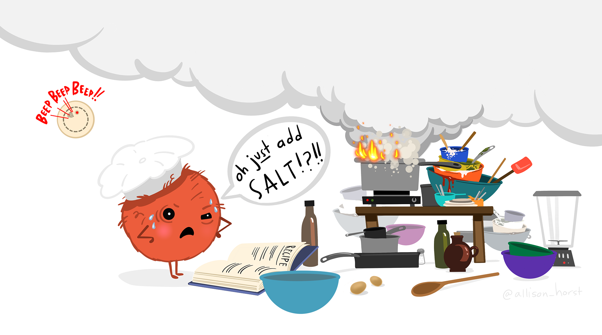
Learn how to keep the kitchen clean.
- Basic tips for reproducible and maintainable data analysis projects
- Project organization
- Coding
- Dependency management
The reproducibility mindset
- Imagine how someone else will see the project for the first time.
Will they be able to understand and use your project?
Practical reproducibility check
Send your project to a colleague and ask them understand and run the code your analysis.
First things first:
📁 Organizing projects
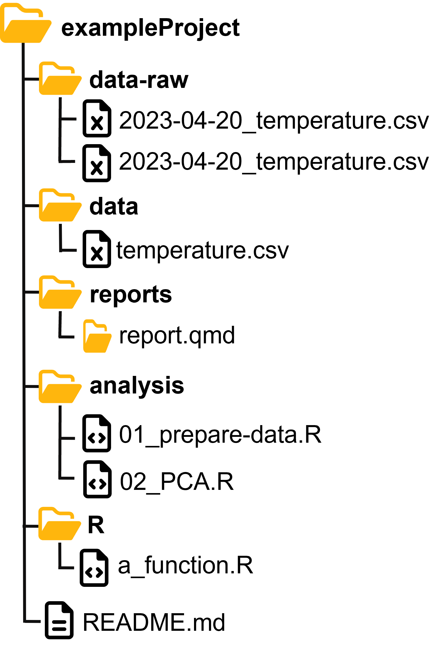
Have a solid project structure
- Self-contained projects: code, data, reports, etc. in one place
- Separate things into folders
- Always include a
READMEfile - Use standard templates (see e.g. the
templateR package)
Name your files properly
Your collaborators and your future self will love you for this.
Principles 1
File names should be
- Machine readable
- Human readable
- Working with default file ordering
1. Machine readable file names
Names should allow for easy searching, grouping and extracting information from file names.
- No space & special characters
- Use consistent separators
Bad examples ❌
📄 2023-04-20 temperature göttingen.csv
📄 2023-04-20 rainfall göttingen.csv
Good examples ✔️
📄 2023-04-20_temperature-goettingen.csv
📄 2023-04-20_rainfall-goettingen.csv
2. Human readable file names
Names shoud be informative and reveal the file content.
- Use separators to make it readable
Bad examples ❌
📄 01preparedataforanalysis.R
📄 01firstscript.R
Good examples ✔️
📄 01_prepare-data-for-analysis.R
📄 01_lm-temperature-trend.R
3. Default ordering
If you order your files by name, the ordering should make sense:
- (Almost) always put something numeric first
- Left-padded numbers (
01,02, …) - Dates in
YYYY-MM-DDformat
- Left-padded numbers (
Chronological order
📄 2023-04-20_temperature-goettingen.csv
📄 2023-04-21_temperature-goettingen.csv
Logical order
📄 01_prepare-data.R
📄 02_lm-temperature-trend.R
💻 Let’s start coding
Use save paths
To read and write files, you need to tell R where to find them.
Common workflow:
Set working directory with setwd(), then read files from there:
This is not reproducible! Your computer at exactly this time is the only one that has this working directory.
Use save paths
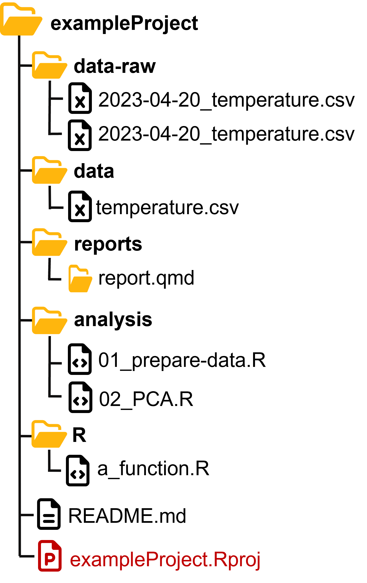
Option 1: Use RStudio projects
- Project root is automatically the working directory
- No need to use
setwd()manually - Read and write files with relative paths:
Create an RStudio Project
From scratch:
File -> New Project -> New Directory -> New Project- Enter a directory name (this will be the name of your project)
- Choose the directory where the project should be initiated
Create Project
Associate an existing folder with an RStudio Project:
File -> New Project -> Existing Directory- Choose your project folder
Create Project
Use save paths
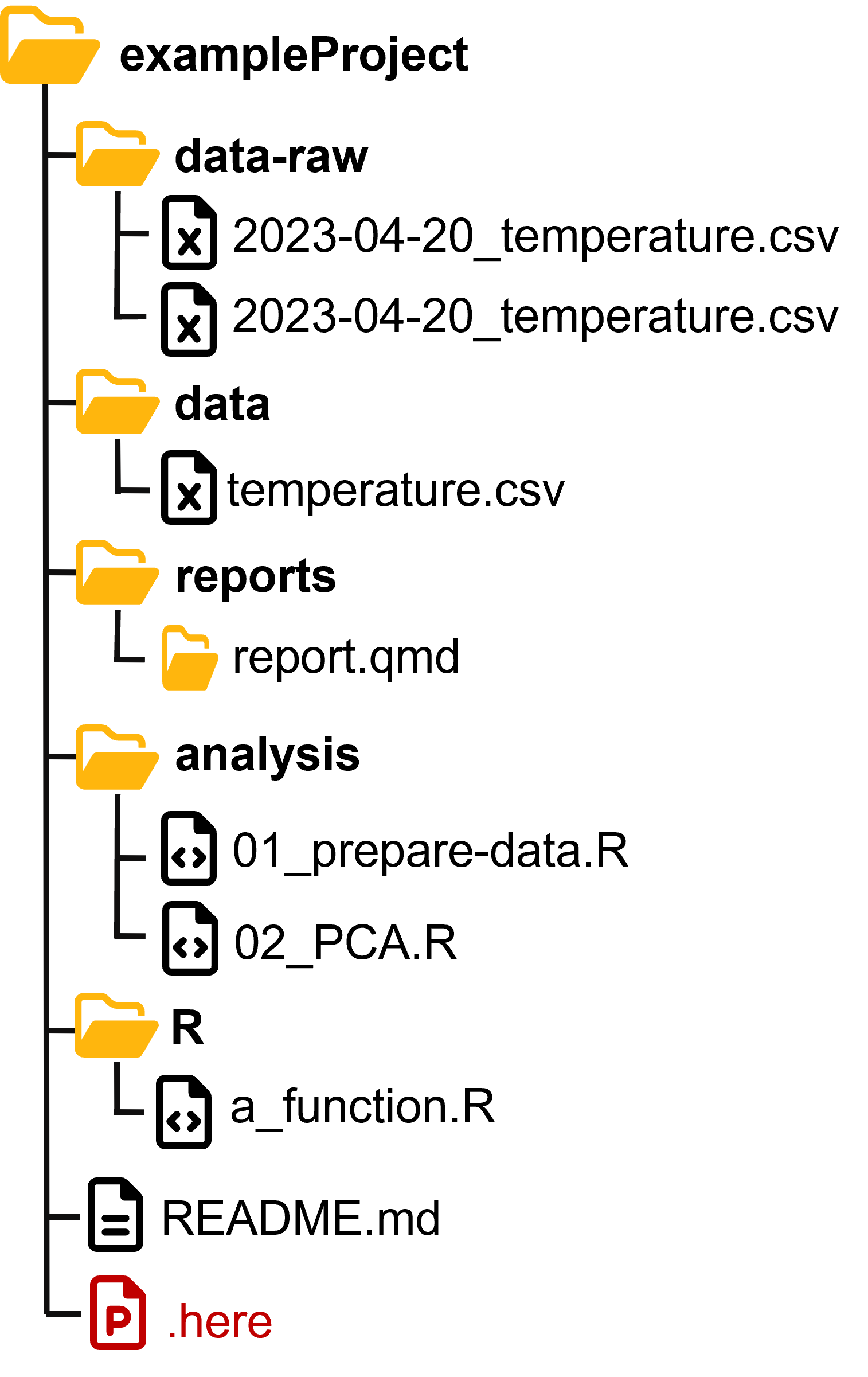
Option 2: Use the here package
- Build your paths using the
herefunction
- Reasonable heuristics to find project files
- Looks for
*.Rproj,.here,.git, … - My recommendation: always use
here- with
*.RprojOR with.here - works in all cases
- with
Write well-structured and consistent code

Artwork by Allison Horst, CC BY 4.0
- This is not about reproducibility, but about readability and maintainability
- Follow standards for consistent and readable code
- For R: tidyverse style guide defines code organization, syntax standards, …
How to structure your scripts
- Use a standardized header
- Initialize at the top
library()calls- global options
- source additional code
- Read all external data in one place
- Why?
- fail fast
- change code in one place
# Purpose: Create Figure 2 showing the relationship
# between body mass and bill length
# Authors: Selina Baldauf, Jane Doe, Jon Doe

# load libraries ---------------------------------
library(tidyverse)
library(vegan)

# Set global options -----------------------------
# Plot themes and colors
theme_set(theme_minimal())
custom_colors <- c("cyan4", "darkorange", "purple")

# Source additional code -------------------------
source("R/my_cool_function.R")

# Read data --------------------------------------
temperature <- read_csv("data/temperature.csv")
rainfall <- read_csv("data/rainfall.csv")
How to structure your scripts
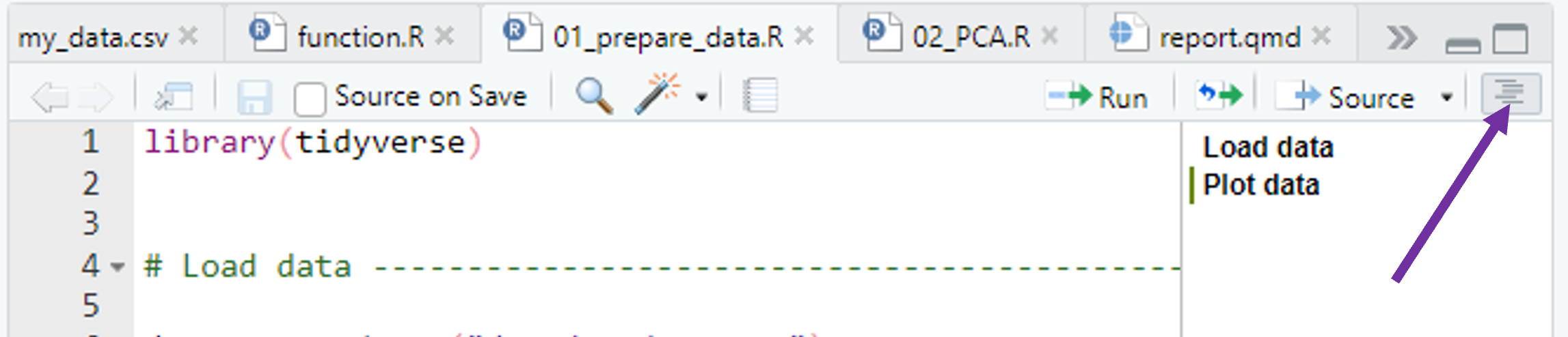
- Use headers to break up your file into sections
- Insert a section label with comment + at least 4
####or----- RStudio keyboard shortcut:
Ctrl/Cmd + Shift + R
- RStudio keyboard shortcut:
How to structure your scripts
- Navigate sections in the file outline
Use a consistent coding style - naming
Have a naming convention for variables and functions and stick to it
- Concise and descriptive (nouns for variables, verbs for functions)
- Consistent capitalization: Use
snake_casefor longer variable names - Avoid conflicts with existing R functions and packages
Use a consistent coding style - spacing
Use a consistent coding style - spacing
- Always put spaces after a comma
- No spaces around parentheses for normal function calls
Use a consistent coding style - spacing
- Always put spaces after a comma
- No spaces around parentheses for normal function calls
- Spaces around most operators (
<-,==,+, etc.)
Use a consistent coding style - spacing
- Always put spaces after a comma
- No spaces around parentheses for normal function calls
- Spaces around most operators (
<-,==,+, etc.) - Spaces before pipes (
|>,%>%) and+in ggplot followed by new line
Use a consistent coding style - spacing
- Always put spaces after a comma
- No spaces around parentheses for normal function calls
- Spaces around most operators (
<-,==,+, etc.) - Spaces before pipes (
|>,%>%) and+in ggplot followed by new line
Use a consistent coding style - width
- Always put spaces after a comma
- No spaces around parentheses for normal function calls
- Spaces around most operators (
<-,==,+, etc.) - Spaces before pipes (
|>,%>%) and+in ggplot followed by new line - Limit your line width to 80 characters.
Use a consistent coding style
Do I really have to remember all of this?
Luckily, no! R and RStudio provide some nice helpers
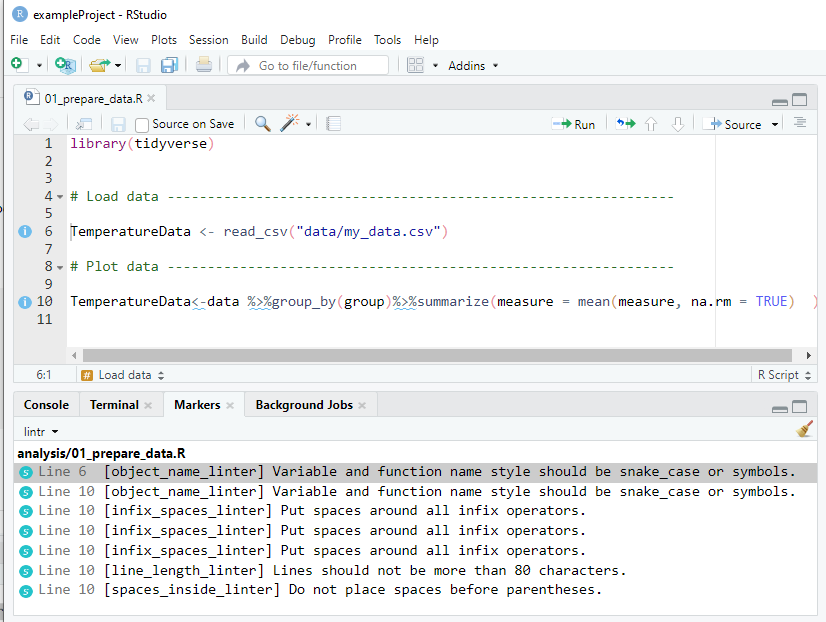
Coding style helpers - {lintr}
The lintr package analyses your code files or entire project and tells you what to fix.
Coding style helpers - lintr
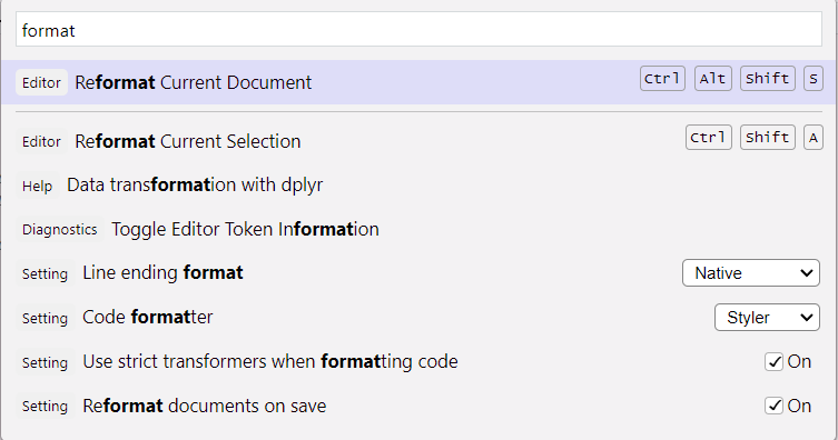
Coding style helpers - Auto-formatting
IDEs offer auto-formatting tools.
Auto-format your scripts on save and let the IDE do the job
RStudio: Open command palette (
Tools->Show command palette), search for “format” -> “Reformat documents on save”
Modularize long scripts
One huge script is hard to maintain
- Break down long scripts into logical units
- Write scripts that do one thing, e.g.
01_prepare-data.R: Read raw data and prepare it for analysis02_run-models.R: Run statistical analysis03_make-figures.R: Create manuscript figures
- Call these scripts sequentially
- Use
source()to source R scripts in other scripts
Modularize long scripts
Write a main workflow script that calls scripts in the right order.
- Often called
make.R,run.Rormain.R
- Gives a nice overview of your workflow
- Very user-friendly: No need to run scripts separately and in the right order
Don’t repeat yourself (DRY)
Example: Same data preparation code for multiple data sets
# Read the data
my_data1 <- readr::read_csv("data/data1.csv")
my_data2 <- readr::read_csv("data/data2.csv")
# Clean and summarize data
my_data1 <- my_data1 |>
  summarize(
    height = mean(height),
    biomass = mean(biomass),
    .by = c(country, species)
  )
my_data2 <- my_data2 |>
  summarize(
    height = mean(height),
    biomass = mean(biomass),
    .by = c(country, species)
  )
What’s the problem?
- What if you need to update the code preparation?
- Bloats the script
Don’t repeat yourself (DRY)
Solution: If you notice that you copy-paste code - write a function
Function in R/prepare_data.R:
🧩 Manage dependencies
Manage dependencies manually
Add the output of devtools::session_info() to your README
─ Session info ───────────────────────────────────────────────────────────────
 setting  value
 version  R version 4.5.2 (2025-10-31 ucrt)
 os       Windows 11 x64 (build 26200)
 system   x86_64, mingw32
 ui       RTerm
 language en
 collate  English_Germany.utf8
 ctype    English_Germany.utf8
 tz       Europe/Berlin
 date     2026-06-16
 pandoc   3.8.3 @ c:\\Program Files\\Positron\\resources\\app\\quarto\\bin\\tools/ (via rmarkdown)
 quarto   NA @ C:\\Users\\Selina\\AppData\\Local\\Programs\\Quarto\\bin\\quarto.exe

─ Packages ───────────────────────────────────────────────────────────────────
 package     * version date (UTC) lib source
 cachem        1.1.0   2024-05-16 [1] CRAN (R 4.5.1)
 cli           3.6.5   2025-04-23 [1] CRAN (R 4.5.1)
 devtools      2.4.5   2022-10-11 [1] CRAN (R 4.5.1)
 digest        0.6.37  2024-08-19 [1] CRAN (R 4.5.1)
 ellipsis      0.3.2   2021-04-29 [1] CRAN (R 4.5.1)
 evaluate      1.0.5   2025-08-27 [1] CRAN (R 4.5.1)
 fastmap       1.2.0   2024-05-15 [1] CRAN (R 4.5.1)
 fs            1.6.6   2025-04-12 [1] CRAN (R 4.5.1)
 glue          1.8.0   2024-09-30 [1] CRAN (R 4.5.1)
 htmltools     0.5.8.1 2024-04-04 [1] CRAN (R 4.5.1)
 htmlwidgets   1.6.4   2023-12-06 [1] CRAN (R 4.5.1)
 httpuv        1.6.16  2025-04-16 [1] CRAN (R 4.5.1)
 jsonlite      2.0.0   2025-03-27 [1] CRAN (R 4.5.1)
 knitr         1.51    2025-12-20 [1] CRAN (R 4.5.2)
 later         1.4.4   2025-08-27 [1] CRAN (R 4.5.1)
 lifecycle     1.0.5   2026-01-08 [1] CRAN (R 4.5.2)
 magrittr      2.0.4   2025-09-12 [1] CRAN (R 4.5.2)
 memoise       2.0.1   2021-11-26 [1] CRAN (R 4.5.1)
 mime          0.13    2025-03-17 [1] CRAN (R 4.5.0)
 miniUI        0.1.2   2025-04-17 [1] CRAN (R 4.5.1)
 otel          0.2.0   2025-08-29 [1] CRAN (R 4.5.2)
 pkgbuild      1.4.8   2025-05-26 [1] CRAN (R 4.5.1)
 pkgload       1.5.0   2026-02-03 [1] CRAN (R 4.5.2)
 profvis       0.4.0   2024-09-20 [1] CRAN (R 4.5.1)
 promises      1.5.0   2025-11-01 [1] CRAN (R 4.5.2)
 purrr         1.2.1   2026-01-09 [1] CRAN (R 4.5.2)
 R6            2.6.1   2025-02-15 [1] CRAN (R 4.5.1)
 Rcpp          1.1.1   2026-01-10 [1] CRAN (R 4.5.2)
 remotes       2.5.0   2024-03-17 [1] CRAN (R 4.5.1)
 rlang         1.1.7   2026-01-09 [1] CRAN (R 4.5.2)
 rmarkdown     2.30    2025-09-28 [1] CRAN (R 4.5.2)
 sessioninfo   1.2.3   2025-02-05 [1] CRAN (R 4.5.1)
 shiny         1.12.1  2025-12-09 [1] CRAN (R 4.5.2)
 urlchecker    1.0.1   2021-11-30 [1] CRAN (R 4.5.1)
 usethis       3.2.1   2025-09-06 [1] CRAN (R 4.5.1)
 vctrs         0.7.1   2026-01-23 [1] CRAN (R 4.5.2)
 xfun          0.56    2026-01-18 [1] CRAN (R 4.5.2)
 xtable        1.8-4   2019-04-21 [1] CRAN (R 4.5.1)
 yaml          2.3.12  2025-12-10 [1] CRAN (R 4.5.2)

 [1] C:/Users/Selina/AppData/Local/Programs/R/R-4.5.2/library

──────────────────────────────────────────────────────────────────────────────
Manage dependencies with {renv}
Idea: Have a project-local environment with all packages needed by the project
- Keep log of the packages and versions you use
- Restore the local project library on other machines
Why this is useful?
- Code will still work even if packages upgrade
- Collaborators can recreate your local project library with one function
- Explicit dependency file states all dependencies
Check out the renv website for more information
Manage dependencies with {renv}
Very simple to use and integrate into your project workflow:
- Others only need to install the
renvpackage, then they can also callrenv::restore()
Conclusion
Take aways
- So many tips and guidelines 😵💫
- Prioritize progress over perfection
- Implement simple things first (e.g. format on save)
- Other guidelines will become habits over time
- Plan ahead
Clean projects and workflows …
… help you to write robust and reproducible code.
Artwork by Allison Horst, CC BY 4.0
Outlook
Of course there is much that I left out:
- Proper documentation
- Version control with Git
- Containerization (e.g. Docker) for full reproducibility
- Using R packages to build a research compendium
- …
But this is for another time
Next lecture
Topic t.b.a.
📅 19th June 🕓 4-5 p.m. 📍 Webex
For topic suggestions and/or feedback send me an email
Thank you for your attention :)
Questions?
References
What they forgot to teach you about R book by Jenny Bryan and Jim Hester
Blogpost by Jenny Bryan on good project-oriented workflows
R best practice blogpost by Krista L. DeStasio
Book about coding style for R: The tidyverse style guide
The Turing way book General concepts and things to think about regarding reproducible research
Selina Baldauf // Reproducible data analysis