library(tidyverse)
#> ── Attaching core tidyverse packages ──────────────────────── tidyverse 2.0.0 ──
#> ✔ dplyr     1.2.0     ✔ readr     2.2.0
#> ✔ forcats   1.0.1     ✔ stringr   1.6.0
#> ✔ ggplot2   4.0.2     ✔ tibble    3.3.1
#> ✔ lubridate 1.9.5     ✔ tidyr     1.3.2
#> ✔ purrr     1.2.1
#> ── Conflicts ────────────────────────────────────────── tidyverse_conflicts() ──
#> ✖ dplyr::filter() masks stats::filter()
#> ✖ dplyr::lag()    masks stats::lag()
#> ℹ Use the conflicted package (<http://conflicted.r-lib.org/>) to force all conflicts to become errorsIntroduction to the tidyverse
Scientific workflows: Tools and Tips 🛠️
2024-02-15
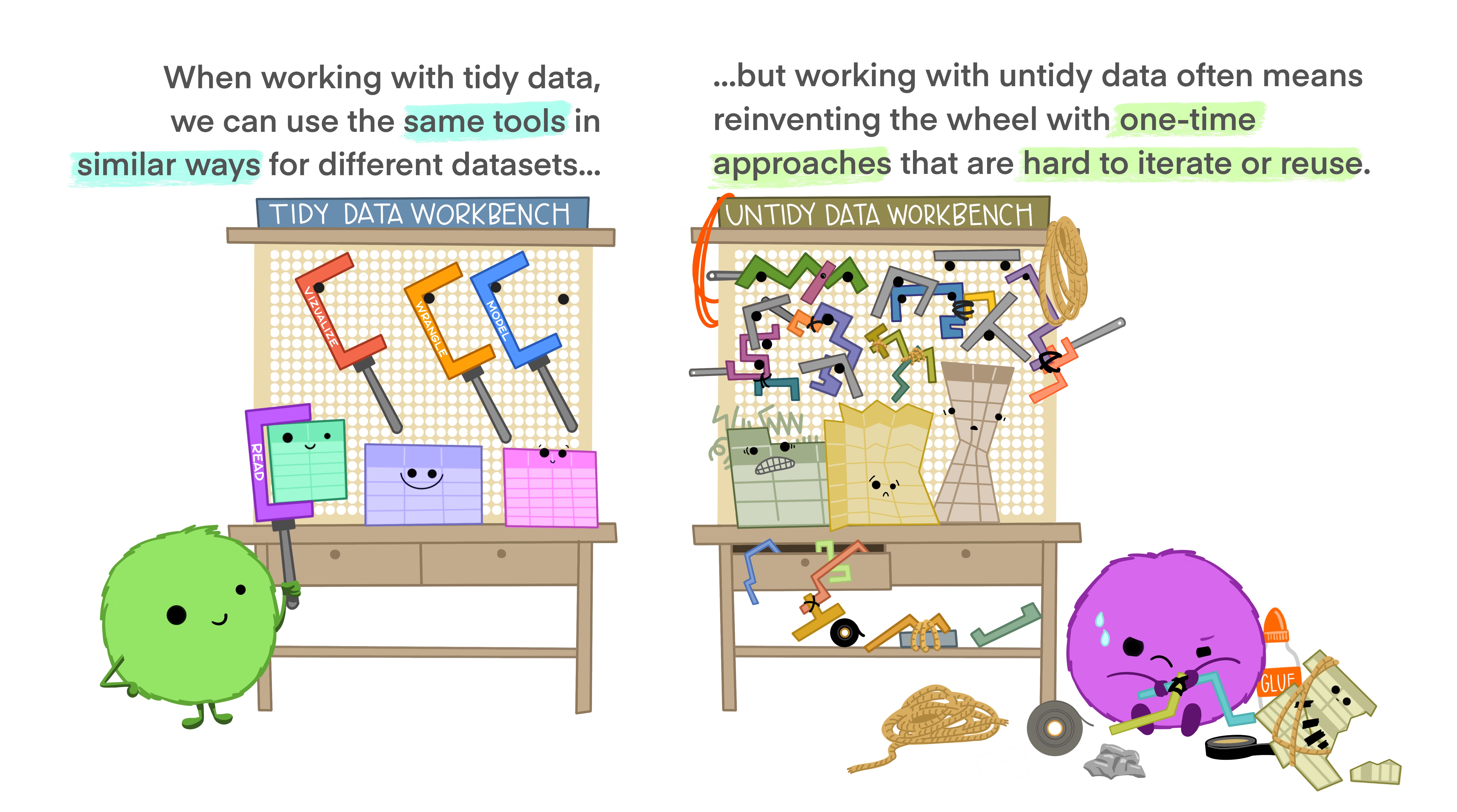
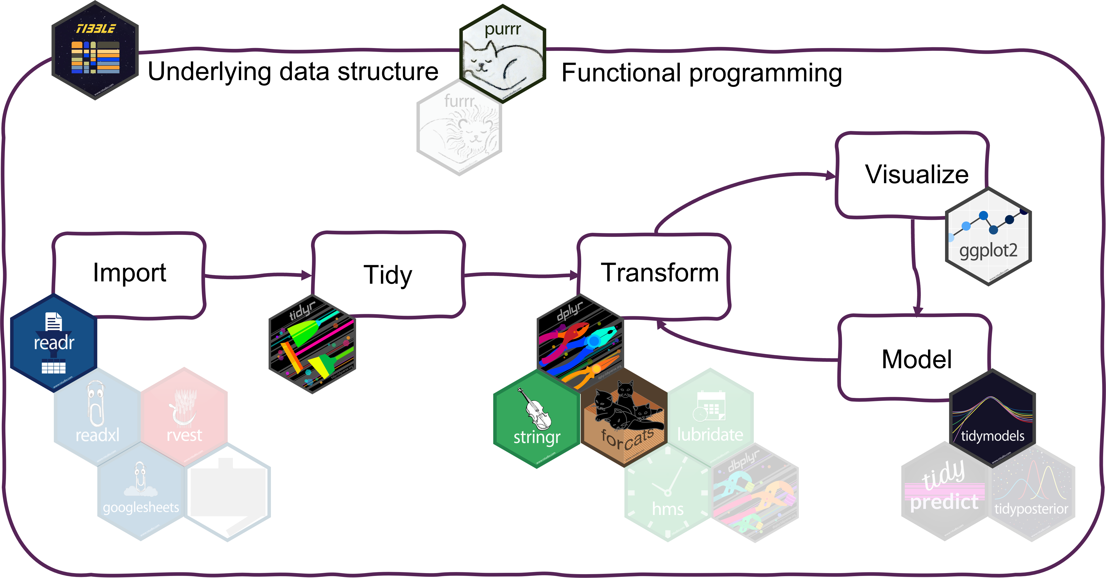
What is the tidyverse?

The tidyverse is an opinionated collection of R packages designed for data science. All packages share an underlying design philosophy, grammar, and data structures.
www.tidyverse.org
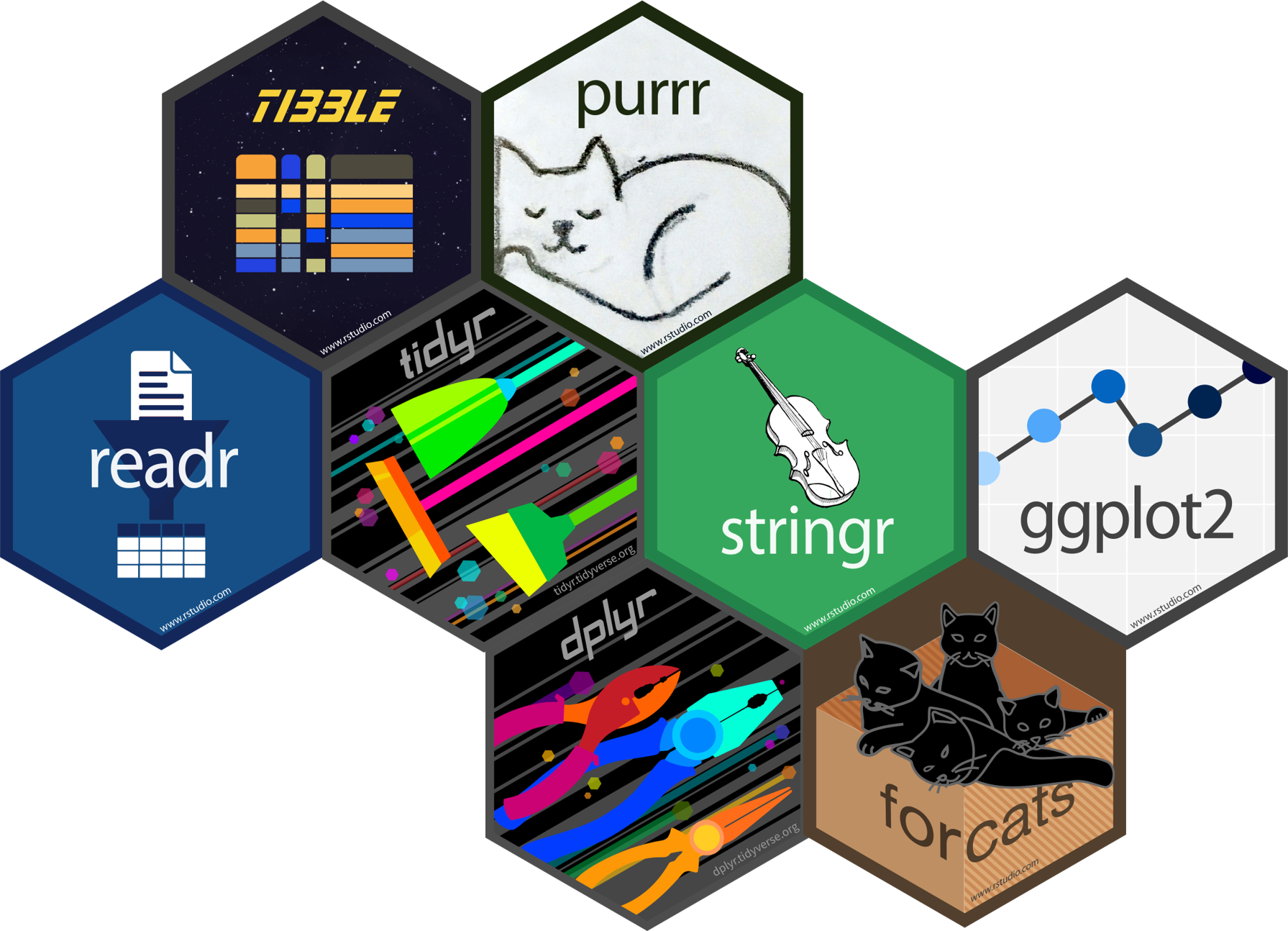
Tidyverse core packages
Why the tidyverse?
Basic idea: Make data analysis efficient and intuitive
- Write code that is easy to read, write and maintain
- More time for data interpretation
- Tidyverse is actively developed and has a large community.
Today
Overview of
- most important packages and functions
- how they work together in a data analysis workflow
- underlying principles of the tidyverse
I can’t show you everything. But the tidyverse has an excellent documentation and cheatsheets.
Which tidyverse packages do you use?
Head over to the menti poll
Data analysis with the tidyverse


![]()


Tibbles from tibble
The underlying data structure
What are tibbles?

Tibbles are
a modern reimagining of the data frame. Tibbles are designed to be (as much as possible) drop-in replacements for data frames.
(Wickham, Advanced R)
Tibbles have the same basic properties as data frames
Everything that you can do with data frames, you can do with tibbles
Main advantage: Tibbles print much nicer to the console
Have a look at this book chapter for a full list of the differences between data frames and tibbles and the advantages of using tibbles.
How to create tibbles?
- Tidyverse functions return tibbles by default
- Create with
tibblefunction (equivalent todata.frame)
How to create tibbles?
Creating a tibble
tibble(
  x = 1:26,
  y = letters,
  z = factor(LETTERS)
)
#> # A tibble: 26 × 3
#>        x y     z
#>    <int> <chr> <fct>
#>  1     1 a     A
#>  2     2 b     B
#>  3     3 c     C
#>  4     4 d     D
#>  5     5 e     E
#>  6     6 f     F
#>  7     7 g     G
#>  8     8 h     H
#>  9     9 i     I
#> 10    10 j     J
#> # ℹ 16 more rows
Creating a data frame
data.frame(
  x = 1:26,
  y = letters,
  z = factor(LETTERS)
)
#>     x y z
#> 1   1 a A
#> 2   2 b B
#> 3   3 c C
#> 4   4 d D
#> 5   5 e E
#> 6   6 f F
#> 7   7 g G
#> 8   8 h H
#> 9   9 i I
#> 10 10 j J
#> 11 11 k K
#> 12 12 l L
#> 13 13 m M
#> 14 14 n N
#> 15 15 o O
#> 16 16 p P
#> 17 17 q Q
#> 18 18 r R
#> 19 19 s S
#> 20 20 t T
#> 21 21 u U
#> 22 22 v V
#> 23 23 w W
#> 24 24 x X
#> 25 25 y Y
#> 26 26 z Z
Import data with readr
Read in your files
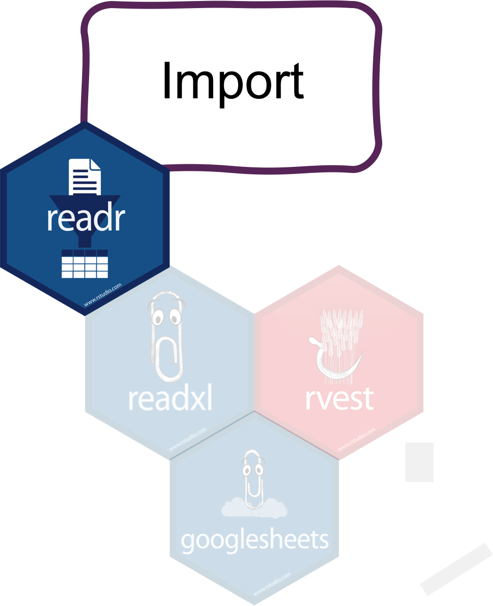
Most important readr functions

read_csvto read comma delimited filesread_tsvto read tab delimited filesread_delimto read files with any delimiter
All read_* functions return a tibble.
Example with arctic temperature data
Data modified from lterdatasampler
arc_weather <- read_csv(file = "data/arc_weather.csv")
arc_weather
#> # A tibble: 365 × 3
#>    date       foolik_mean_temp_c poolik_mean_temp_c
#>    <date>                  <dbl>              <dbl>
#>  1 1988-06-01                8.4              11.8
#>  2 1988-06-02                6                 8.90
#>  3 1988-06-03                5.8               8.14
#>  4 1988-06-04                1.8               3.95
#>  5 1988-06-05                6.8               9.81
#>  6 1988-06-06                5.2               8.74
#>  7 1988-06-07                2.2               6.11
#>  8 1988-06-08                9.4              12.1
#>  9 1988-06-09               13.1              16.5
#> 10 1988-06-10               17.7              20.9
#> # ℹ 355 more rows
Advantages of readr
Faster than
read.table/read.csvBetter defaults than base R (e.g. guessing of data types)
Returns tibbles
Tidyverse packages for other data types:
readxlfor Excel fileshavenfor SPSS, SAS, and Stata filesgooglesheets4for Google sheets- …
Tidy data with tidyr
Reorganize the data

What is tidy data?
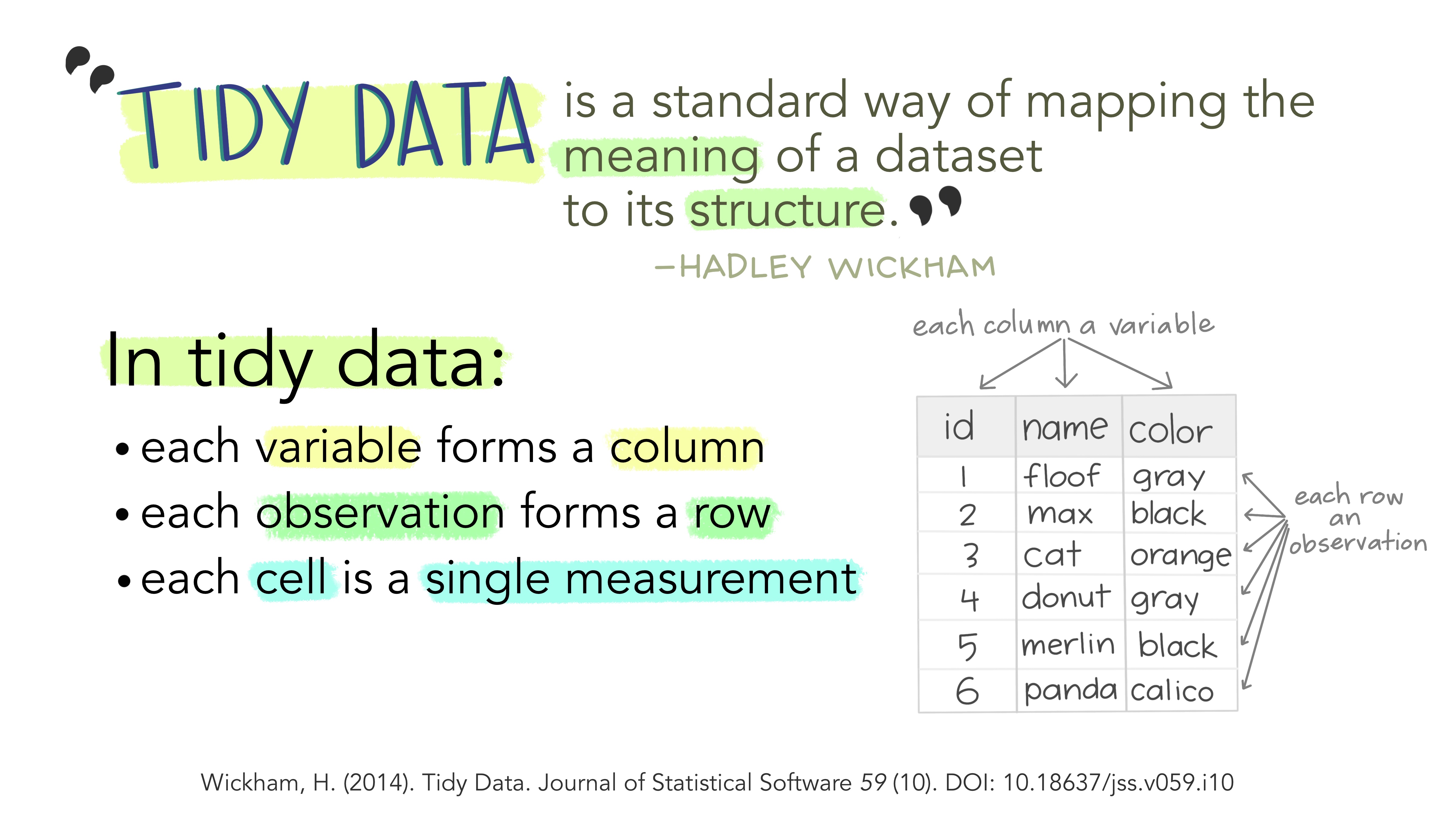
Advantages of tidy data
The main advantages of tidy data is that the tidyverse packages are built to work with it.
Tidy data with tidyr

Tidyrreorganizes the data but does not change values- Most important functionality:
- Pivoting:
pivot_longerandpivot_wider - Splitting and combining columns:
separate_wider_delim/position/regexandunite - Handle missing values:
drop_na,replace_na,complete
- Pivoting:
Example
What is not tidy about our weather data?
arc_weather
#> # A tibble: 365 × 3
#>    date       foolik_mean_temp_c poolik_mean_temp_c
#>    <date>                  <dbl>              <dbl>
#>  1 1988-06-01                8.4              11.8
#>  2 1988-06-02                6                 8.90
#>  3 1988-06-03                5.8               8.14
#>  4 1988-06-04                1.8               3.95
#>  5 1988-06-05                6.8               9.81
#>  6 1988-06-06                5.2               8.74
#>  7 1988-06-07                2.2               6.11
#>  8 1988-06-08                9.4              12.1
#>  9 1988-06-09               13.1              16.5
#> 10 1988-06-10               17.7              20.9
#> # ℹ 355 more rows- Each row has multiple observations
- Variables are split across multiple columns
Example
This can be solved with pivot_longer
pivot_longer(arc_weather,
  cols = c(foolik_mean_temp_c, poolik_mean_temp_c))
#> # A tibble: 730 × 3
#>    date       name               value
#>    <date>     <chr>              <dbl>
#>  1 1988-06-01 foolik_mean_temp_c  8.4
#>  2 1988-06-01 poolik_mean_temp_c 11.8
#>  3 1988-06-02 foolik_mean_temp_c  6
#>  4 1988-06-02 poolik_mean_temp_c  8.90
#>  5 1988-06-03 foolik_mean_temp_c  5.8
#>  6 1988-06-03 poolik_mean_temp_c  8.14
#>  7 1988-06-04 foolik_mean_temp_c  1.8
#>  8 1988-06-04 poolik_mean_temp_c  3.95
#>  9 1988-06-05 foolik_mean_temp_c  6.8
#> 10 1988-06-05 poolik_mean_temp_c  9.81
#> # ℹ 720 more rows
Example
You can also directly name the new columns:
arc_weather <- pivot_longer(arc_weather,
  cols = c(foolik_mean_temp_c, poolik_mean_temp_c),
  names_to = "station",
  values_to = "mean_temp_c")
arc_weather
#> # A tibble: 730 × 3
#>    date       station            mean_temp_c
#>    <date>     <chr>                    <dbl>
#>  1 1988-06-01 foolik_mean_temp_c        8.4
#>  2 1988-06-01 poolik_mean_temp_c       11.8
#>  3 1988-06-02 foolik_mean_temp_c        6
#>  4 1988-06-02 poolik_mean_temp_c        8.90
#>  5 1988-06-03 foolik_mean_temp_c        5.8
#>  6 1988-06-03 poolik_mean_temp_c        8.14
#>  7 1988-06-04 foolik_mean_temp_c        1.8
#>  8 1988-06-04 poolik_mean_temp_c        3.95
#>  9 1988-06-05 foolik_mean_temp_c        6.8
#> 10 1988-06-05 poolik_mean_temp_c        9.81
#> # ℹ 720 more rows
Transform data with dplyr
How to actually change values
![]()
Transform data with dplyr

Data cleaning, adding new columns, summarizing, …
Depending on the data type in combination with
stringrfor character columnslubridatefor date-time columnsforcatsfor factor columns
Data cleaning and filtering
select picks variables (columns) based on their names
select(arc_weather,
  date, mean_temp_c)
#> # A tibble: 730 × 2
#>    date       mean_temp_c
#>    <date>           <dbl>
#>  1 1988-06-01        8.4
#>  2 1988-06-01       11.8
#>  3 1988-06-02        6
#>  4 1988-06-02        8.90
#>  5 1988-06-03        5.8
#>  6 1988-06-03        8.14
#>  7 1988-06-04        1.8
#>  8 1988-06-04        3.95
#>  9 1988-06-05        6.8
#> 10 1988-06-05        9.81
#> # ℹ 720 more rows
filter picks observations (rows) based on their values
filter(arc_weather,
  station == "foolik_mean_temp_c")
#> # A tibble: 365 × 3
#>    date       station            mean_temp_c
#>    <date>     <chr>                    <dbl>
#>  1 1988-06-01 foolik_mean_temp_c         8.4
#>  2 1988-06-02 foolik_mean_temp_c         6
#>  3 1988-06-03 foolik_mean_temp_c         5.8
#>  4 1988-06-04 foolik_mean_temp_c         1.8
#>  5 1988-06-05 foolik_mean_temp_c         6.8
#>  6 1988-06-06 foolik_mean_temp_c         5.2
#>  7 1988-06-07 foolik_mean_temp_c         2.2
#>  8 1988-06-08 foolik_mean_temp_c         9.4
#>  9 1988-06-09 foolik_mean_temp_c        13.1
#> 10 1988-06-10 foolik_mean_temp_c        17.7
#> # ℹ 355 more rows
Combine filter with other packages
lubridate to filter by month
# Filter rows from May
filter(arc_weather,
  month(date) == 5)
#> # A tibble: 62 × 3
#>    date       station            mean_temp_c
#>    <date>     <chr>                    <dbl>
#>  1 1989-05-01 foolik_mean_temp_c      -3.3
#>  2 1989-05-01 poolik_mean_temp_c      -0.312
#>  3 1989-05-02 foolik_mean_temp_c      -0.8
#>  4 1989-05-02 poolik_mean_temp_c       2.20
#>  5 1989-05-03 foolik_mean_temp_c       0.5
#>  6 1989-05-03 poolik_mean_temp_c       2.59
#>  7 1989-05-04 foolik_mean_temp_c      -2.1
#>  8 1989-05-04 poolik_mean_temp_c       0.457
#>  9 1989-05-05 foolik_mean_temp_c      -2
#> 10 1989-05-05 poolik_mean_temp_c       1.19
#> # ℹ 52 more rows
stringr to filter characters
# Filter rows where the station contains "foolik"
filter(arc_weather,
  str_detect(station, "foolik"))
#> # A tibble: 365 × 3
#>    date       station            mean_temp_c
#>    <date>     <chr>                    <dbl>
#>  1 1988-06-01 foolik_mean_temp_c         8.4
#>  2 1988-06-02 foolik_mean_temp_c         6
#>  3 1988-06-03 foolik_mean_temp_c         5.8
#>  4 1988-06-04 foolik_mean_temp_c         1.8
#>  5 1988-06-05 foolik_mean_temp_c         6.8
#>  6 1988-06-06 foolik_mean_temp_c         5.2
#>  7 1988-06-07 foolik_mean_temp_c         2.2
#>  8 1988-06-08 foolik_mean_temp_c         9.4
#>  9 1988-06-09 foolik_mean_temp_c        13.1
#> 10 1988-06-10 foolik_mean_temp_c        17.7
#> # ℹ 355 more rows
Change and add values
Add columns with mutate
# Add column with temperature in K
mutate(arc_weather,
  mean_temp_k = mean_temp_c + 274.15)
#> # A tibble: 730 × 4
#>    date       station            mean_temp_c mean_temp_k
#>    <date>     <chr>                    <dbl>       <dbl>
#>  1 1988-06-01 foolik_mean_temp_c        8.4         283.
#>  2 1988-06-01 poolik_mean_temp_c       11.8         286.
#>  3 1988-06-02 foolik_mean_temp_c        6           280.
#>  4 1988-06-02 poolik_mean_temp_c        8.90        283.
#>  5 1988-06-03 foolik_mean_temp_c        5.8         280.
#>  6 1988-06-03 poolik_mean_temp_c        8.14        282.
#>  7 1988-06-04 foolik_mean_temp_c        1.8         276.
#>  8 1988-06-04 poolik_mean_temp_c        3.95        278.
#>  9 1988-06-05 foolik_mean_temp_c        6.8         281.
#> 10 1988-06-05 poolik_mean_temp_c        9.81        284.
#> # ℹ 720 more rows
Change and add values
Change the values of existing columns with mutate
# Remove _mean_temp_c from station
arc_weather <- mutate(arc_weather,
                        station = str_remove(station, "_mean_temp_c"))
arc_weather
#> # A tibble: 730 × 3
#>    date       station mean_temp_c
#>    <date>     <chr>         <dbl>
#>  1 1988-06-01 foolik         8.4
#>  2 1988-06-01 poolik        11.8
#>  3 1988-06-02 foolik         6
#>  4 1988-06-02 poolik         8.90
#>  5 1988-06-03 foolik         5.8
#>  6 1988-06-03 poolik         8.14
#>  7 1988-06-04 foolik         1.8
#>  8 1988-06-04 poolik         3.95
#>  9 1988-06-05 foolik         6.8
#> 10 1988-06-05 poolik         9.81
#> # ℹ 720 more rows
Summarize data
summarize will collapse the data to a single row
# Calculate the overall mean temperature
summarize(arc_weather,
            overall_mean = mean(mean_temp_c, na.rm = TRUE))
#> # A tibble: 1 × 1
#>   overall_mean
#>          <dbl>
#> 1        -7.10
Summarizing data by group
summarize in combination with group_by will collapse the data to a single row per group
# Calculate the mean temperature for each station
arc_weather_group <- group_by(arc_weather, station)
summarize(arc_weather_group,
  overall_mean = mean(mean_temp_c, na.rm = TRUE))
#> # A tibble: 2 × 2
#>   station overall_mean
#>   <chr>          <dbl>
#> 1 foolik         -8.60
#> 2 poolik -5.60group_bycan be used for any dplyr function to perform the operation by group
The pipe |>
Data transformation often requires multiple operations in sequence.
The pipe operator |> helps to keep these operations clear and readable.
- You may also see
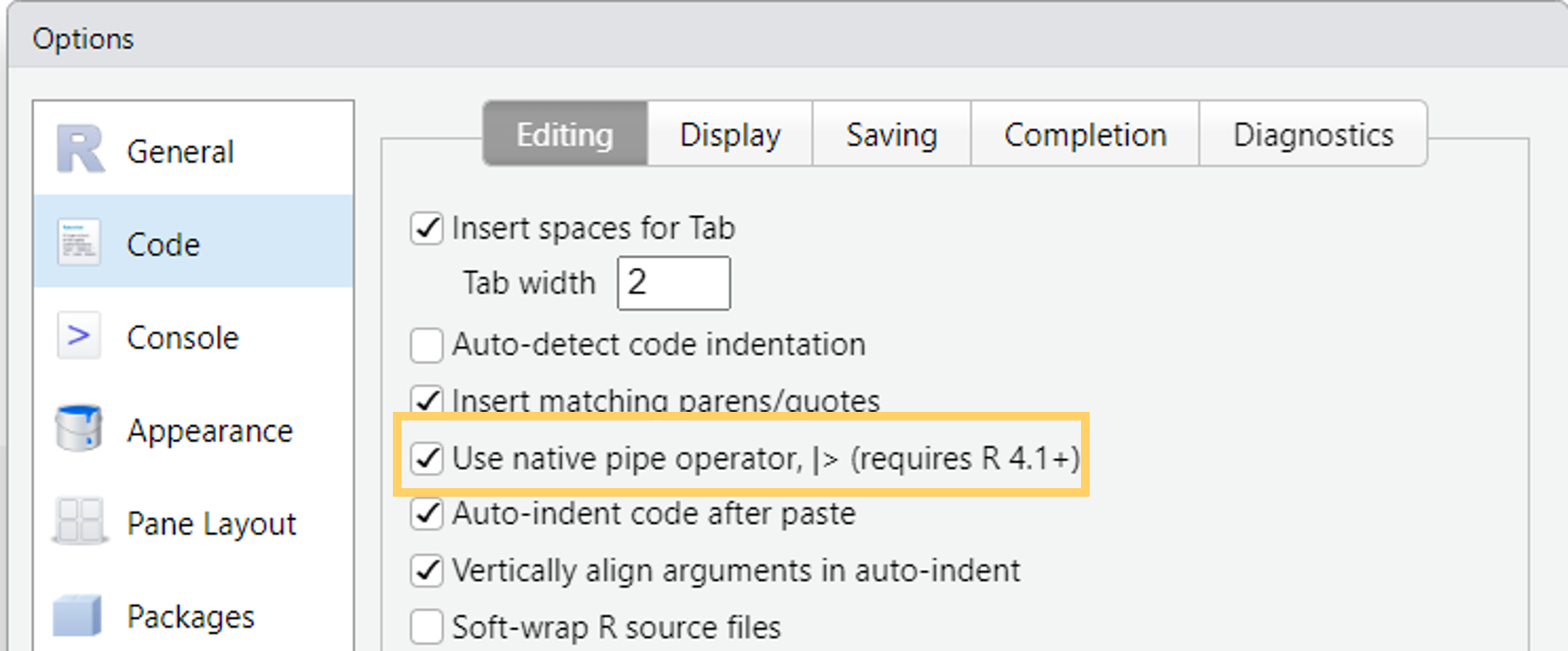
%>%from themagrittrpackage (tidyverse) - Turn on the native R pipe
|>in Tools -> Global Options -> Code
Visualize data with ggplot2
Quick exploratory plots and data masterpieces
A ggplot showcase

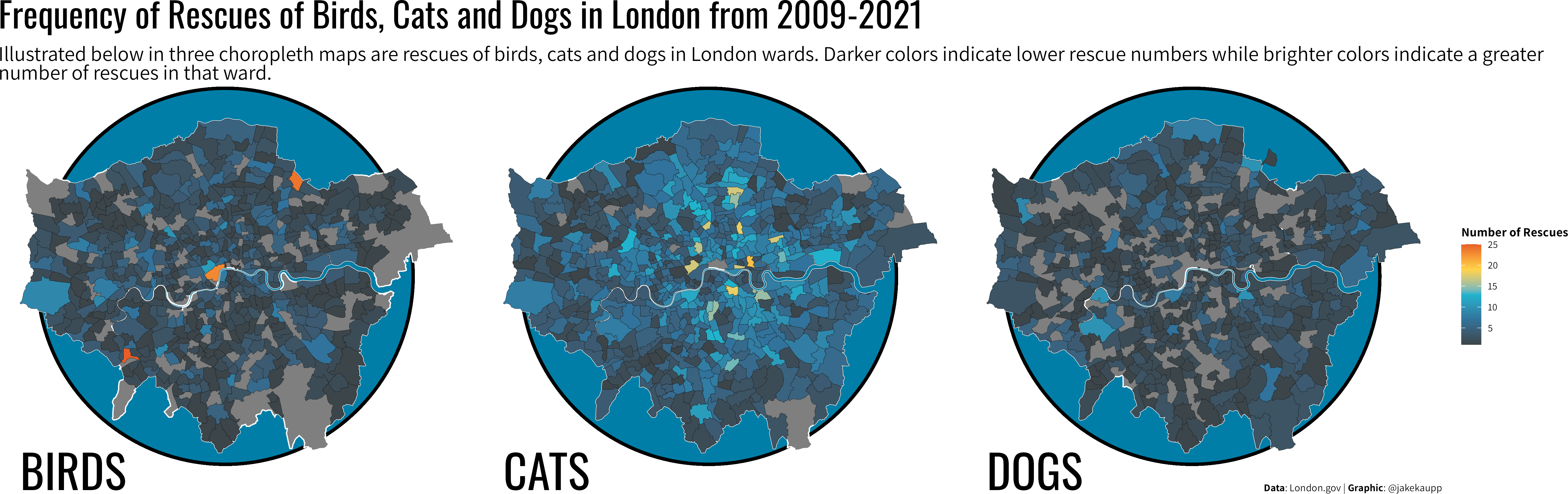
A ggplot showcase
A ggplot showcase
Advantages of ggplot
- Consistent grammar
- Flexible structure allows you to produce any type of plots
- Highly customizable appearance (themes)
- Many extension packages that provide additional plot types, themes, colors, animation, …
- Find a list of ggplot extensions here
- Perfect package for exploratory data analysis and beautiful plots
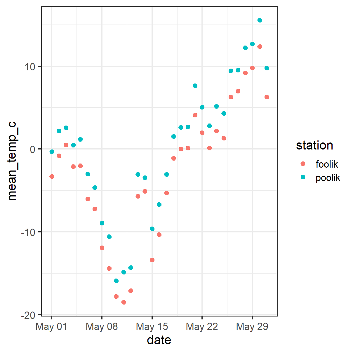
Basic ggplot
Basic idea: Stack layers of the plot on top of each other with +
arc_weather_may <- filter(arc_weather,
  month(date) == 5)
ggplot(data = arc_weather_may,
  aes(
    x = date,
    y = mean_temp_c,
    color = station
)) +
geom_point()- aesthetics define how data variables are mapped onto plot properties
- geoms define the type of plot (e.g. points, lines, bars, …)
Basic ggplot
- Gplot offers many more customization options and layers
- Works well with the pipe
|>
arc_weather |>
  filter(month(date) == 5) |>
  ggplot(aes(
    x = date,
    y = mean_temp_c,
    color = station)) +
  geom_point() +
  geom_smooth() +
  labs(
    title = "Mean temperature in May",
    x = "Date",
    y = "Mean temperature (°C)") +
  scale_color_viridis_d()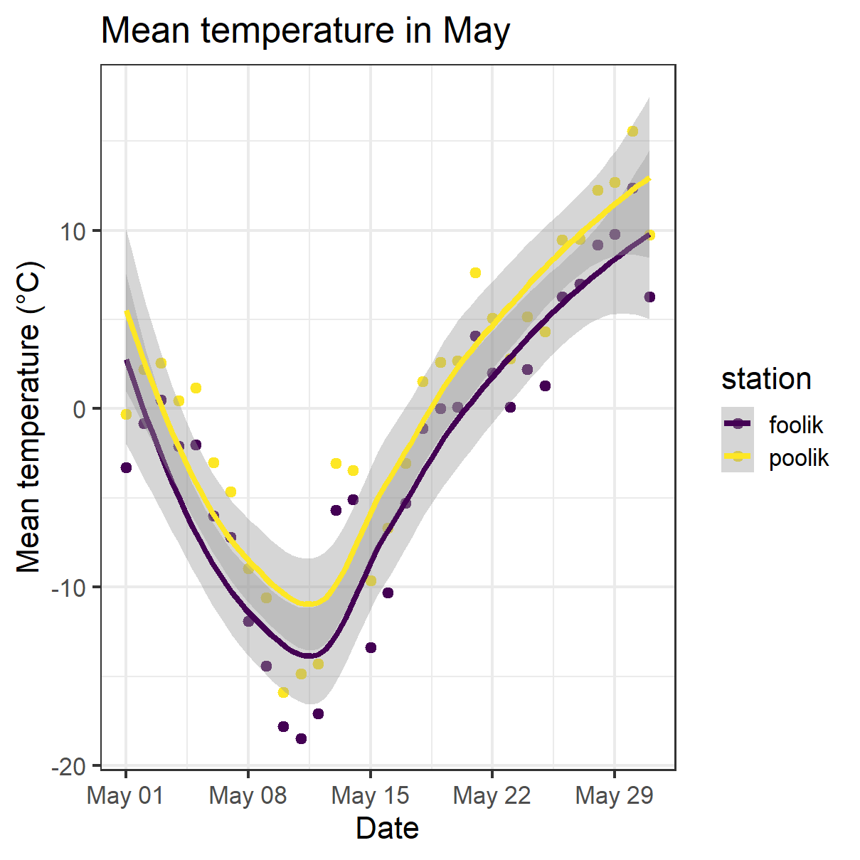
Functional programming with purrr

Functional programming with purrr

- Apply functions to multiple elements of a list/vector/…
- Replace e.g. for loops/apply-functions
- Often
purrrfunctions are more intuitive - See here for a full comparison between base R functions and purr functions
- Most important function:
map- Comes in different versions, depending on the input and the desired output
A simple example
Draw 4 numbers from normal distribution with means 1, 2, 3, 4.
Do it by hand
# Do it by hand
set.seed(123)
rnorm(n = 4, mean = 1, sd = 1)
#> [1] 0.4395244 0.7698225 2.5587083 1.0705084
rnorm(n = 4, mean = 2, sd = 1)
#> [1] 2.1292877 3.7150650 2.4609162 0.7349388
rnorm(n = 4, mean = 3, sd = 1)
#> [1] 2.313147 2.554338 4.224082 3.359814
rnorm(n = 4, mean = 4, sd = 1)
#> [1] 4.400771 4.110683 3.444159 5.786913
Use purrr
# Use purrr
set.seed(123)
means <- 1:4
samples <- map(means, rnorm, n = 4, sd = 1)
str(samples)
#> List of 4
#>  $ : num [1:4] 0.44 0.77 2.56 1.07
#>  $ : num [1:4] 2.129 3.715 2.461 0.735
#>  $ : num [1:4] 2.31 2.55 4.22 3.36
#>  $ : num [1:4] 4.4 4.11 3.44 5.79
Different versions of the map function
These are just some examples, there are many more options:
| Output | Input | Purr function |
|---|---|---|
| List | 1 Vector | map |
| List | 2 Vectors | map2 |
| Vector of desired type | 1 Vector | map_lgl |
| Vector of desired type | 2 Vectors | map2_lgl |
| Data frame | 1 Vector | map_df |
| Data frame | 2 Vectors | map2_df |
A more complex example
Read in and analyse multiple files with the same structure at once.
# Step 1: List all files in your data directory
paths <- list.files("data")
#> [1] "foolik.csv" "poolik.csv"# Step 2: Read all files into a list of tibbles
arc_weather_files <- map(paths, read_csv)
arc_weather_files
#> [[1]]
#> # A tibble: 365 × 3
#> date station mean_temp_c
#> <date> <chr> <dbl>
#> 1 1988-06-01 foolik 8.4
#> 2 1988-06-02 foolik 6
#> 3 1988-06-03 foolik 5.8
#> 4 1988-06-04 foolik 1.8
#> 5 1988-06-05 foolik 6.8
#> 6 1988-06-06 foolik 5.2
#> 7 1988-06-07 foolik 2.2
#> 8 1988-06-08 foolik 9.4
#> 9 1988-06-09 foolik 13.1
#> 10 1988-06-10 foolik 17.7
#> # ℹ 355 more rows
#>
#> [[2]]
#> # A tibble: 365 × 3
#> date station mean_temp_c
#> <date> <chr> <dbl>
#> 1 1988-06-01 poolik 11.5
#> 2 1988-06-02 poolik 8.00
#> 3 1988-06-03 poolik 8.50
#> 4 1988-06-04 poolik 4.31
#> 5 1988-06-05 poolik 9.56
#> 6 1988-06-06 poolik 8.10
#> 7 1988-06-07 poolik 5.56
#> 8 1988-06-08 poolik 12.7
#> 9 1988-06-09 poolik 16.0
#> 10 1988-06-10 poolik 21.5
#> # ℹ 355 more rowsA more complex example
Read in and analyse multiple files with the same structure at once.
# Step 3: Apply a linear model to each station file,
# get the model summary of each model and extract the coefficients
arc_weather_files |>                             # Take the data
  map(\(x) lm(mean_temp_c ~ date, data = x)) |>  # Apply the same model to every tibbel in the list
  map(summary) |>                                # Get the model summary of both models
  map_dbl("r.squared")                           # Extract the r-squared from the model summaries
#> [1] 0.2018279 0.2000210
Summary
Summary
Where to get started with the tidyverse?
- Check out the lecture website for links to documenation, cheatsheets and book